Arch Instability
6 min read • 1,189 wordsSeveral nonlinear static analysis methods are used to investigate instabilities in a shallow arch.
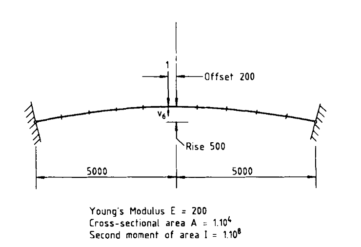
 In this problem, we investigate how this programmatic interface can be used to solve a highly nonlinear problem.Consider the shallow arch shown above (Clarke and Hancock, 1990).This problem exhibits several critical points along the solution path,and requires the use of a sophisticated algorithm to properly traverse these.In this study, we will investigate how the OpenSees framework can be used to compose these algorithms.We will perform the analysis by creating a
 xara.Model object, and usingits methods to perform various tasks. A method is simply a function thatis linked to a particular instance of a data structure. In this case, the Modeldata structure holds the geometry and state (i.e., the current values of solution variables) of our structural model. Some methods that you might see being used in this notebook include (you wont need to make any changes to the use of any of these):-
Model.integrator(...)This method configures the iteration strategy to be performed in the next increment
-
Model.analyze(n)This method appliesnincrements, and between each increment, performs Newton-Raphson iterations.
Model data structure is created by the arch_model helper function, which we load from the file
arch.py:
We’ll also find the following imports convenient:from arch import arch_model
import numpy as np
import matplotlib.pyplot as plt

try:
    plt.style.use("veux-web")
except:
    pass
Solution Strategy
Our general strategy is implemented in the following functionsolve().This function adopts an incremental approachwhere the load is applied in small steps of varying size.The arguments to the function are:model: axara.Modelinstance
node: an integer indicating which node to collect results from.
arch_model helper function mentionedabove.
def analyze(model, mid, increment, steps, dx, *args):
    # Initialize some variables
    xy = [[0,0]]      # Container to hold solution history (i.e., load factor and displacement at `node`)
    status = 0   # Convergence flag; Model.analyze() will return 0 if successful.

    # Configure the first load increment strategy; explained below
    increment(model, dx, *args)

    steps = 1000
    i = 0
    while  model.getTime() < 2000 and i < steps:
        i += 1
    # for step in range(steps):

        # 1. Perform Newton-Raphson iterations until convergence for 1 load
        #    increment
        status = model.analyze(1)

        # 2. Store the displacement and load factor
        xy.append([model.nodeDisp(mid, 2), model.getTime()])

        # 3. If the iterations failed, try cutting
        #    the initial increment in half
        if status != 0:
            dx /= 2
            increment(model, dx, *args)

    return np.array(xy).T
The strategies used by Clarke and Hancock are:def create_figure(): fig, ax = plt.subplots(1, 1, figsize=(6, 4)) ax.axhline(0, color='black', lw=0.5) ax.axvline(0, color='black', lw=0.5) ax.set_title("Displacement vs Load Factor") ax.set_ylabel(r"Load factor $\lambda$") ax.set_xlabel("Displacement $u$") ax.set_xlim([0, 1200]) ax.set_ylim([-800, 3000]) return ax
- Solution 1
-
Iterative strategy: Constant load (Section 3.1)
Load incrementation strategy: Direct incrementation of the load parameter (Section 4.1.1) - Solution 2
-
Iterative strategy: Constant vertical displacement under the load,
(Section 3.2)
Load incrementation strategy: Incrementation of the displacement component (Section 4.1.2) - Solution 3
-
Iterative strategy: Constant arc-length (Section 3.3)
Load incrementation strategy: Incrementation of the arc-length (Section 4.1.3) - Solution 4
-
Iterative strategy: Minimum unbalanced displacement norm (Section 3.5)
Load incrementation strategy: Incrementation of the arc-length (Section 4.1.3) - Solution 5
-
Iterative strategy: Constant weighted response (Section 3.7, equation (39))
Load incrementation strategy: Incrementation of the arc-length (Section 4.1.3) - Solution 6
-
Iterative strategy: Minimum unbalanced force norm (Section 3.6)
Load incrementation strategy: Using the current stiffness parameter (Section 4.2, equation (57)) - Solution 7
-
Iterative strategy: Minimum unbalanced force norm (Section 3.6)
Load incrementation strategy: Incrementation of the arc-length (Section 4.1.3) - Solution 8
-
Iterative strategy: Constant arc-length (Section 3.3)
Load incrementation strategy: Using the current stiffness parameter (Section 4.2, equation (57))
Load Control
def solution0(model, dx):
    model.integrator("LoadControl", 400.0)
ax = create_figure()

x, y = analyze(*arch_model(), solution0, 6, 400.0)
ax.plot(-x, y, '-x', label="S0");

def solution1(model, dx):
    Jd = 5
    Jmax = 15
    model.integrator("LoadControl", dx, Jd, -800., 800.)
ax = create_figure()
x, y = analyze(*arch_model(), solution1, None, 400.0)
ax.plot(-x, y, '-o', label="S1")
[]

Displacement Control
def solution2(model,  dx, mid, dof, dumin=None, dumax=None):
    Jd  = 5
    if dumin is not None:
        model.integrator("DisplacementControl", mid, dof, dx, Jd, dumin, dumax)
    else:
        model.integrator("DisplacementControl", mid, dof, dx, Jd)
ax = create_figure()
model, mid = arch_model()
x, y = analyze(model, mid, solution2,    7, -150, *(mid, 2, -300, -10))
ax.plot(-x, y, '.-', label="S2")
[]

def norm_control(model, dx, *args):
    Jd  = 5
    model.integrator("MinUnbalDispNorm",  dx, Jd, -15, 10, det=True)
ax = create_figure()
x, y = analyze(*arch_model(), norm_control,  None, 10)
ax.plot(-x, y, "-", label="norm")
[]

def arc_control(model, dx, *args,  a=0):
    model.integrator("ArcLength", dx, a, det=True, exp=0.5, reference="point")
ax = create_figure()
fig = ax.figure

x, y = analyze(*arch_model(), solution0, 6, 400.0)
ax.plot(-x, y, 'x', label="S0")

x, y = analyze(*arch_model(), solution1, 6, 400.0)
ax.plot(-x, y, 'x', label="S1")


model, mid = arch_model()
x, y = analyze(model, mid, solution2,    7, -150, *(mid, 2))
ax.plot(-x, y, 'o', label="S2")

x, y = analyze(*arch_model(), solution2,  536, -1.5, *(mid, 2))
ax.plot(-x, y, '-', label="S2")

# x, y = analyze(*arch_model(), arc_control, 9500, 0.5, 0)
# ax.plot(-x, y, "-", label="arc")


x, y = analyze(*arch_model(), norm_control,  7000, 1.0)
ax.plot(-x, y, "-", label="norm")

x, y = analyze(*arch_model(), arc_control, None,  45)
ax.plot(-x, y, ".", label="arc")

# x, y = analyze(*arch_model(), arc_control,  80,  88, 0)
# ax.plot(-x, y, "+", label="arc")

# x, y = analyze(*arch_model(), arc_control,  80, 188, 0)
# ax.plot(-x, y, "*", label="arc")

# x, y = analyze(*arch_model(), arc_control, 8000, 0.8, 0)
# ax.plot(-x, y, "x", label="arc")


fig.legend();

fix, ax = plt.subplots()
ax.plot(-x, '.');
ax.set_title("Displacement vs Step Number")
ax.set_ylabel("Displacement $u$")
ax.set_xlabel("Analysis step $n$");

The following animation of the solution is created in
Animating.ipynb
References
Clarke, M.J. and Hancock, G.J. (1990) ‘A study of incremental‐iterative strategies for non‐linear analyses’, International Journal for Numerical Methods in Engineering, 29(7), pp. 1365–1391. Available at: https://doi.org/10.1002/nme.1620290702 .
The source code for creating the arch structure is given below:
# ===----------------------------------------------------------------------===//
#
#         OpenSees - Open System for Earthquake Engineering Simulation
#                Structural Artificial Intelligence Laboratory
#
# ===----------------------------------------------------------------------===//
#
import numpy as np
import xara

# Create the model
def arch_model():

    # Define model parameters
    L      = 5000
    Rise   = 500
    Offset = 200

    # Compute radius
    R  = Rise/2 + (2*L)**2/(8*Rise)
    th = 2*np.arcsin(L/R)

    #
    # Build the model
    #
    model = xara.Model(ndm=2, ndf=3)

    # Create nodes
    ne  = 10
    nen =  2             # nodes per element
    nn  = ne*(nen-1)+1
    mid = (nn+1)//2      # midpoint node

    for i, angle in enumerate(np.linspace(-th/2, th/2, nn)):
        tag = i + 1

        # Compute x and add offset if midpoint
        x = R*np.sin(angle)
        if tag == mid:
            x -= Offset

        # Compute y
        y = R*np.cos(angle)

        # create the node
        model.node(tag, x, y)

    # Define elastic section properties
    E = 200
    A = 1e4
    I = 1e8
    model.section("ElasticFrame", 1, A=A, E=E, I=I)

    # Create elements
    transf = 1
    model.geomTransf("Corotational", transf)
    for i in range(ne):
        tag   = i+1
        nodes = (i+1, i+2)
        model.element("PrismFrame", tag, nodes, section=1, transform=transf)


    model.fix( 1, 1, 1, 0)
    model.fix(nn, 1, 1, 0)

    # Create a load pattern that scales linearly
    model.pattern("Plain", 1, "Linear")

    # Add a nodal load to the pattern
    model.load(mid, 0.0, -1.0, 0.0, pattern=1)


    # Select linear solver, and ensure determinants are
    # computed and stored.
    # model.system("ProfileSPD")
    # model.system("FullGeneral")
    # model.system("BandGeneral", det=True)
    # model.system("Umfpack", det=True)

    model.test("NormUnbalance", 1e-6, 25, 9)
    model.algorithm("Newton")
    model.analysis("Static")


    return model, mid