Moment-Curvature Analysis

A reinforced concrete cross-section is modeled using a fiber section, and a moment-curvature analysis is performed.

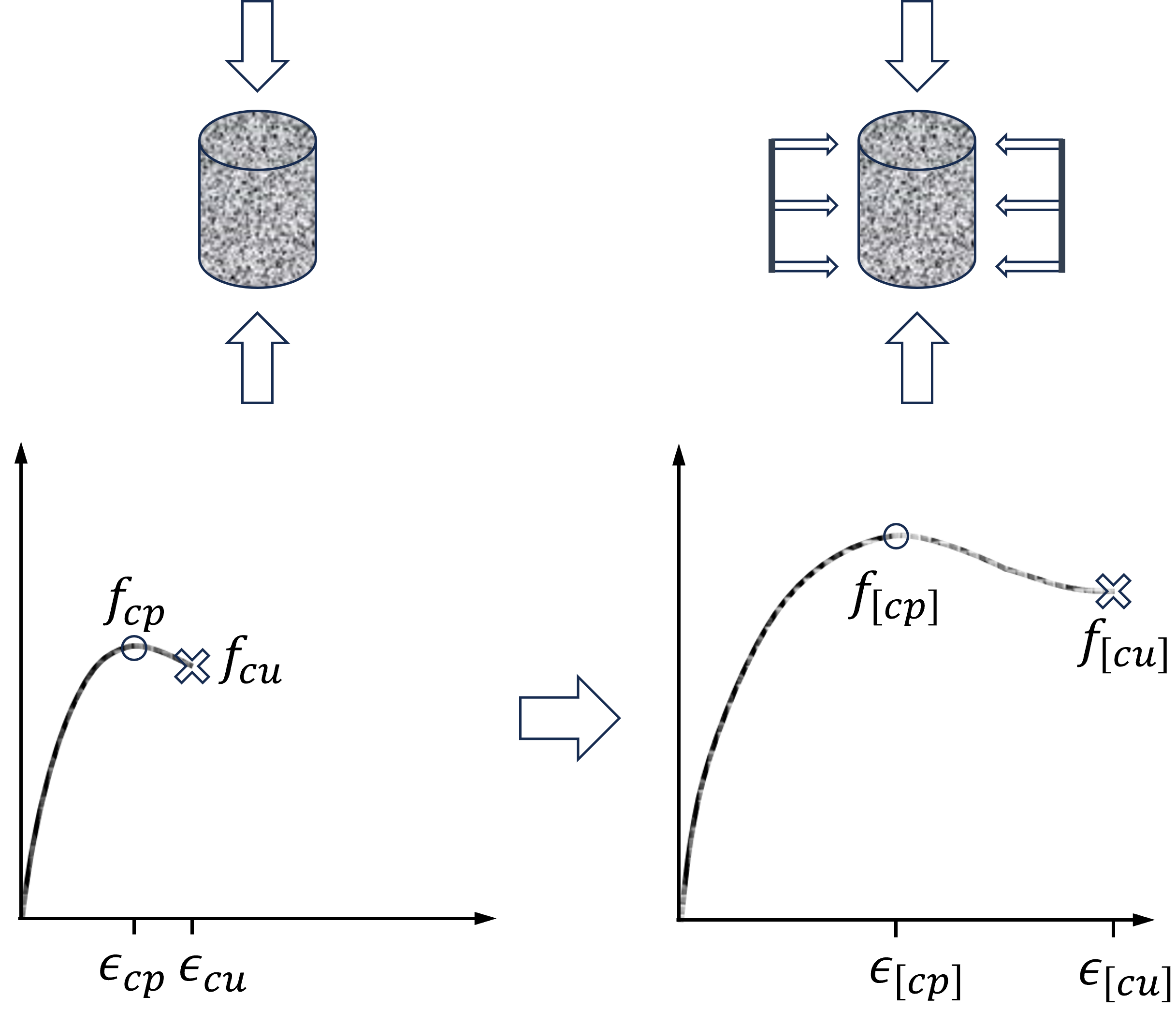
This example performs a moment-curvature analysis of a reinforced concrete section which is represented by a fiber discretization. Because we are only interested in the response quantities of the cross section, a zero-length element is used to wrap the cross section.

  
import veux
import numpy as np

import xara.units.fks as units
from xara.units.fks import kip, ksi

from xsection.library import from_aisc
from xsection.analysis import SectionInteraction

import matplotlib.pyplot as plt
plt.style.use("veux-web")

Steel  

  

shape = from_aisc("W14x426", units=units)
veux.render(shape.model)

  
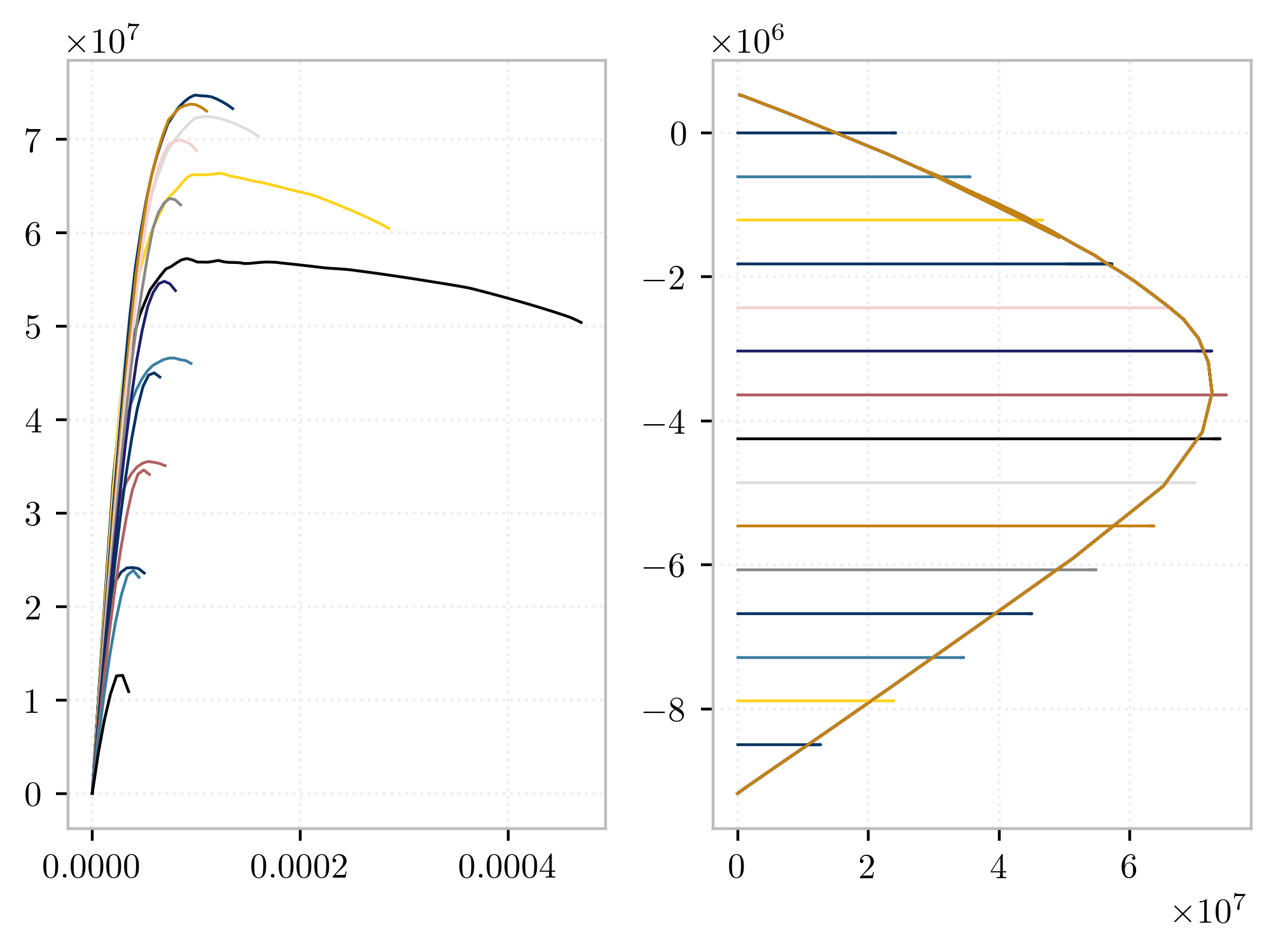
steel = {
        "type": "J2",
        "nu": 0.3,
        "E":  29000*ksi,
        "Fy":    50*ksi,
        "Hiso": 0.003*29e3*ksi,
        "Fs": 0, "Fo": 0, "Hsat": 16
}

Ny = shape.area*steel["Fy"]

axial = np.linspace(-Ny, Ny, 10)

si = SectionInteraction(("ShearFiber", shape, steel), axial=axial)

fig, ax = plt.subplots(1,2, figsize=(10, 5), sharey=True)

for N, M, k in si.moment_curvature():
    ax[0].plot(k, M, '-') #, label=f"{N/kip:.0f} kip")
    ax[1].plot([N/Ny], [M[-1]], '.')


ax[0].axvline(0, color="k", lw=1)
ax[0].axhline(0, color="k", lw=1)
ax[1].axvline(0, color="k", lw=1)
ax[1].axhline(0, color="k", lw=1)
ax[0].set_xlabel("Curvature, $\\kappa$")
ax[0].set_ylabel("Moment, $M(\\varepsilon, \\kappa)$")
ax[1].set_xlabel("Axial force, $N/N_y$");

Concrete  

  
from xsection.library import Rectangle, Circle
from xsection import CompositeSection

h = 24
b = 15
d = 7/8
r = 0 #d/2

c = 1.5

bar = Circle(d/2, z=2, mesh_scale=1/2, divisions=4, name="rebar")

shape = CompositeSection([
            Rectangle(    b, h,     z=0, name="cover"),
            Rectangle(b-2*c, h-2*c, z=1, name="core"),
            *bar.linspace([-b/2+c+r, -h/2+c+r], [ b/2-c-r,-h/2+c+r], 3), # Top bars
            *bar.linspace([-b/2+c+r,        0], [ b/2-c-r,       0], 2), # Center bars
            *bar.linspace([-b/2+c+r,  h/2-c-r], [ b/2-c-r, h/2-c-r], 3)  # Bottom bars
        ])


print(shape.summary())

artist = veux.create_artist(shape.model) #veux.model.FiberModel(shape.create_fibers()))
# artist.draw_samples()
artist.draw_outlines()
artist.draw_surfaces()
artist

  
from xara.units.iks import kip, ksi

mat = [
    { # Confined
        "name": "core",
        "type": "Concrete01",
        "Fc":   6*ksi,
        "ec0":  0.004,
        "Fcu":  5*ksi,
        "ecu":  0.014,
    },
    { # Unconfined
        "name": "cover",
        "type": "Concrete01",
        "Fc":  -5*ksi,
        "ec0": -0.002,
        "Fcu":  0,
        "ecu": -0.006,
    },
    {
        "name": "rebar",
        "type": "Steel01",
        "E":   30e3*ksi,
        "Fy":    60*ksi,
        "b":   0.01
    }
]

axial = np.linspace(-1200*kip, 250*kip, 15)

si = SectionInteraction(("Fiber", shape, mat), axial=axial)

fig, ax = plt.subplots(1,2, sharey=True, constrained_layout=True, figsize=(10, 5))
mmax = []

for n, m, k in si.moment_curvature():
    ax[0].plot(k, m, '-')

    # ax[1].plot([n]*len(m), m, '-', lw=0.3, markersize=0.5)
    ax[1].plot([n], [max(m)], 'o')

ax[0].axvline(0, color="k", lw=1)
ax[0].axhline(0, color="k", lw=1)
ax[1].axvline(0, color="k", lw=1)
ax[1].axhline(0, color="k", lw=1)
ax[0].set_xlabel("Curvature, $\\kappa$")
ax[0].set_ylabel("Moment, $M(\\varepsilon, \\kappa)$")
ax[1].set_xlabel("Axial force, $P$");

Modeling  

The figure below shows the fiber discretization for the section.

The dimensions of the fiber section are shown below. The section depth is 24 inches, the width is 15 inches, and there are 1.5 inches of cover around the entire section.

Strong axis bending is about the section $z$ -axis. The section is separated into confined and unconfined concrete regions, for which separate fiber discretizations will be generated. Reinforcing steel bars will be placed around the boundary of the confined and unconfined regions. The fiber discretization for the section is shown below.

A fiber section is created by grouping various patches and layers:

Note in Python you must pass the section tag when calling patch and layer

model.section("Fiber", 1)
# Create the concrete core fibers
model.patch("rect", 1, 10, 1, cover-y1, cover-z1, y1-cover, z1-cover, section=1)
# Create the concrete cover fibers (top, bottom, left, right, section=1)
model.patch("rect", 2, 10, 1, -y1, z1-cover, y1, z1, section=1)
model.patch("rect", 2, 10, 1, -y1, -z1, y1, cover-z1, section=1)
model.patch("rect", 2,  2, 1, -y1, cover-z1, cover-y1, z1-cover, section=1)
model.patch("rect", 2,  2, 1,  y1-cover, cover-z1, y1, z1-cover, section=1)
# Create the reinforcing fibers (left, middle, right, section=1)
model.layer("straight", 3, 3, As, y1-cover, z1-cover, y1-cover, cover-z1, section=1)
model.layer("straight", 3, 2, As, 0.0, z1-cover, 0.0, cover-z1, section=1)
model.layer("straight", 3, 3, As, cover-y1, z1-cover, cover-y1, cover-z1, section=1)

section Fiber 1 {

    # Create the concrete core fibers
    patch rect 1 10 1 [expr $cover-$y1] [expr $cover-$z1] [expr $y1-$cover] [expr $z1-$cover]

    # Create the concrete cover fibers (top, bottom, left, right)
    patch rect 2 10 1  [expr -$y1] [expr $z1-$cover] $y1 $z1
    patch rect 2 10 1  [expr -$y1] [expr -$z1] $y1 [expr $cover-$z1]
    patch rect 2  2 1  [expr -$y1] [expr $cover-$z1] [expr $cover-$y1] [expr $z1-$cover]
    patch rect 2  2 1  [expr $y1-$cover] [expr $cover-$z1] $y1 [expr $z1-$cover]

    # Create the reinforcing fibers (left, middle, right)
    layer straight 3 3 $As [expr $y1-$cover] [expr $z1-$cover] [expr $y1-$cover] [expr $cover-$z1]
    layer straight 3 2 $As 0.0 [expr $z1-$cover] 0.0 [expr $cover-$z1]
    layer straight 3 3 $As [expr $cover-$y1] [expr $z1-$cover] [expr $cover-$y1] [expr $cover-$z1]
}    

The model consists of two nodes and a ZeroLengthSection element. A depiction of the element geometry is shown in figure  zerolength. The drawing on the left of figure  zerolength shows an edge view of the element where the local $z$ -axis, as seen on the right side of the figure and in figure  rcsection0, is coming out of the page. Node 1 is completely restrained, while the applied loads act on node 2. A compressive axial load, $P$ , of $180$ kips is applied to the section during the moment-curvature analysis.

For the zero length element, a section discretized by concrete and steel is created to represent the resultant behavior. UniaxialMaterial objects are created to define the fiber stress-strain relationships: confined concrete in the column core, unconfined concrete in the column cover, and reinforcing steel.

Analysis  

The section analysis is performed by the procedure moment_curvature defined in the file MomentCurvature.tcl for Tcl, and Example2.1.py for Python. The arguments to the procedure are the tag secTag of the section to be analyzed, the axial load axialLoad applied to the section, the maximum curvature maxK, and the number numIncr of displacement increments to reach the maximum curvature.

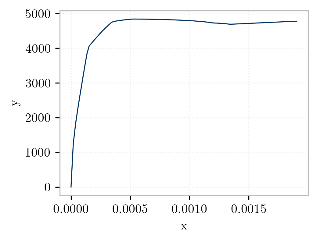
The output for the moment-curvature analysis will be the section forces and deformations, stored in the file section1.out. In addition, an estimate of the section yield curvature is printed to the screen.

In the moment_curvature procedure, the nodes are defined to be at the same geometric location and the ZeroLengthSection element is used. A single load step is performed for the axial load, then the integrator is changed to DisplacementControl to impose nodal displacements, which map directly to section deformations. A reference moment of 1.0 is defined in a Linear time series. For this reference moment, the DisplacementControl  integrator will determine the load factor needed to apply the imposed displacement.

The load factor is the moment, and the nodal rotation is the curvature of the element with zero thickness.

The expected output is:

Estimated yield curvature: 0.000126984126984

The file section1.out contains for each committed state a line with the load factor and the rotation at node 3. This can be used to plot the moment-curvature relationships shown below.