Simply Supported Solid Beam

In this example a simply supported beam is modelled with two dimensional solid elements.

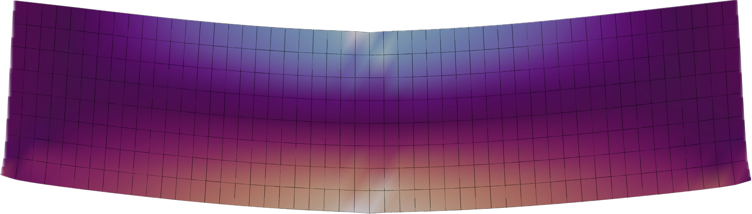
In this example a simply supported beam is modelled with two dimensional solid elements.

Each node of the analysis has two displacement degrees of freedom. Thus the model is defined with ndm = 2 and ndf = 2.

model -ndm 2 -ndf 2

import opensees.openseespy as ops

model = ops.Model(ndm=2, ndf=2)

This is a plane strain problem, and the elastic isotropic material is used.

material ElasticIsotropic   1   1000   0.25  [expr 6.75/(12.0*32.174)]
section PlaneStrain 1 1 2.0

#                                 tag  E      nu      rho
model.material("ElasticIsotropic", 1, 1000.0, 0.25, 6.75/g)
model.section("PlaneStrain", 1, material=1, thickness=2.0)

A mesh is generated using the block2D command. The number of nodes in the local $x$ -direction of the block is $nx$ and the number of nodes in the local $y$ -direction of the block is $ny$ . The block2D generation nodes {1,2,3,4} are prescribed to define the two dimensional domain of the beam, which is of size $40\times10$ .

block2D $nx $ny   1 1  $Quad  $eleArgs {
    1   0   0
    2  40   0
    3  40  10
    4   0  10
}

surface = model.surface((nx, ny),
              element=element, args=args,
              points={
                1: [  0.0,  0.0],
                2: [ 40.0,  0.0],
                3: [ 40.0, 10.0],
                4: [  0.0, 10.0]
              })

Three different quadrilateral elements can be used for the analysis. These may be created using the names "BbarQuad", "EnhancedQuad" or "Quad".

For initial gravity load analysis, a single load pattern with a linear time series and two vertical nodal loads are used.

A solution algorithm of type Newton is used for the problem. The solution algorithm uses a ConvergenceTest which tests convergence on the norm of the energy increment vector. Ten static load steps are performed.

Dynamic Analysis  

Following the static analysis, the wipeAnalysis and remove loadPatern commands are used to remove the nodal loads and create a new analysis. The nodal displacements have not changed. However, with the external loads removed the structure is no longer in static equilibrium.

The integrator for the dynamic analysis if of type GeneralizedMidpoint with $\alpha = 0.5$ . This choice is uconditionally stable and energy conserving for linear problems. Additionally, this integrator conserves linear and angular momentum for both linear and non-linear problems. The dynamic analysis is performed using $100$ time increments with a time step $\Delta t = 0.50$ .

The results consist of the file Node.out, which contains a line for every time step. Each line contains the time and the vertical displacement at the bottom center of the beam. The time history is shown in Figure 1.