Dynamic Shell Analysis

Finite element analysis of a shell model using OpenSees and veux.

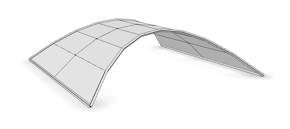
In this example a simple problem in shell dynamics is considered. The structure is a curved hoop shell structure that looks like the roof of a Safeway.

Renderings are created from the script render.py, which uses the veux  Python package.

Modeling  

For shell analysis, a typical shell element is defined as a surface in three dimensional space. Each node of a shell analysis has six degrees of freedom, three displacements and three rotations. Thus the model is defined with ndm = 3 and ndf = 6.

model -ndm 3 -ndf 6

import opensees.openseespy as ops

model = ops.Model(ndm=3, ndf=6)

The shell element is constructed using the ShellMITC4 formulation. An elastic membrane-plate material section model is constructed using the section command and the "ElasticShell"  formulation. In this case, the elastic modulus $E = 3.0e3$ , Poisson’s ratio $\nu = 0.25$ , the thickness $h = 1.175$ and the mass density per unit volume $\rho = 1.27$

#                                           tag E   nu     h    rho
model.section("ElasticShell", 1, E, 0.25, 1.175, 1.27)

# create the material
section ElasticShell  1   3.0e3  0.25  1.175  1.27

A mesh is generated using the surface()  function. The number of nodes in the local $x$ -direction of the block is nx and the number of nodes in the local $y$ -direction of the block is ny.

# generate the nodes and elements
block2D $nx $ny 1 1 $element $eleArgs {
    1   -20    0     0
    2   -20    0    40
    3    20    0    40
    4    20    0     0
    5   -10   10    20 
    7    10   10    20   
    9     0   10    20 
} 

# generate the surface nodes and elements
surface = model.surface((nx, ny),
              element="ShellMITC4", args=(1,),
              points={
                  1: [-20.0,  0.0,  0.0],
                  2: [-20.0,  0.0, 40.0],
                  3: [ 20.0,  0.0, 40.0],
                  4: [ 20.0,  0.0,  0.0],
                  5: [-10.0, 10.0, 20.0],
                  7: [ 10.0, 10.0, 20.0],
                  9: [  0.0, 10.0, 20.0]
              })

The surface function generates nodes with tags {1,2,3,4, 5,7,9}.

Boundary conditions are applied using the fixZ  command. In this case, all the nodes whose $z$ -coordiate is $0.0$ have the boundary condition {1,1,1, 0,1,1}: all degrees-of-freedom are fixed except rotation about the x-axis, which is free. The same boundary conditions are applied where the $z$ -coordinate is $40.0$ .

For initial gravity load analysis, a single load pattern with a linear time series and three vertical nodal loads are used. A solution algorithm of type Newton is used for the problem. Five static load steps are performed. A scaled rendering of the deformed shape under gravity loading is shown below:

artist = veux.render(model, model.nodeDisp,
                     canvas="gltf",
                     scale=200,
                     reference={"plane.outline"},
                     displaced={"plane.surface", "plane.outline"},
)

veux.serve(artist)

Dynamic Analysis  

After the static analysis, the wipeAnalysis and remove loadPatern commands are used to remove the nodal loads and create a new analysis. The nodal displacements have not changed. However, with the external loads removed the structure is no longer in static equilibrium.

The integrator for the dynamic analysis if of type GeneralizedMidpoint with $\alpha = 0.5$ . This choice is uconditionally stable and energy conserving for linear problems. Additionally, this integrator conserves linear and angular momentum for both linear and non-linear problems. The dynamic analysis is performed using $250$ time increments with a time step $\Delta t = 0.50$ .

The results consist of the file Node.out, which contains a line for every time step. Each line contains the time and the vertical displacement at the upper center of the hoop structure. The time history is shown in the figure below.