Continuum Cantilever

Dynamic analysis of a cantilever beam, modeled with 8-node brick elements.

Each node of the analysis has three displacement degrees of freedom. Thus the model is defined with ndm = 3 and ndf = 3.

model -ndm 3 -ndf 3

import xara

model = xara.Model(ndm=3, ndf=3)

The finite element mesh is generated using the block3D  method. The first three arguments, nx, ny, and nz specify the number of nodes to be generated in the $x$ , $y$ , and $z$ directions. For this example a mesh of $2 \times 2 \times 10$ elements is produced. The next two arguments specify from where to begin generating element and node tags. The sixth argument element is a string which selects the type of element to be generated, and the seventh argument eleArgs is a tuple  of arguments to be passed to each element that is created. The final argument of the block3D command is a block specifying the location of up to 8 reference nodes.

# mesh generation
block3D $nx $ny $nz   1 1  $element  $args {
    1   -1     -1      0
    2    1     -1      0
    3    1      1      0
    4   -1      1      0 
    5   -1     -1     10
    6    1     -1     10
    7    1      1     10
    8   -1      1     10
}

model.block3D((nx, ny, nz), (1, 1), "Brick", 1, {
              1: [-1.0, -1.0,  0.0],
              2: [ 1.0, -1.0,  0.0],
              3: [ 1.0,  1.0,  0.0],
              4: [-1.0,  1.0,  0.0],
              5: [-1.0, -1.0, 10.0],
              6: [ 1.0, -1.0, 10.0],
              7: [ 1.0,  1.0, 10.0],
              8: [-1.0,  1.0, 10.0]})

Two possible brick elements can be used for the analysis. These may be created using either StdBrick or BbarBrick. An elastic isotropic material is used.

For initial gravity load analysis, a single load pattern with a linear time series and a single nodal loads is used.

Boundary conditions are applied using the fixZ command. In this case, all the nodes whose $z$ -coordiate is $0.0$ have the boundary condition {1,1,1}, fully fixed.

A solution algorithm of type Newton is used for the problem. The solution algorithm uses a ConvergenceTest which tests convergence on the norm of the energy increment vector. Five static load steps are performed.

Dynamics  

Following the static analysis, the wipeAnalysis and remove commands are used to remove the nodal loads and create a new analysis. The nodal displacements have not changed. However, with the external loads removed the structure is no longer in static equilibrium.

The integrator for the dynamic analysis if of type GeneralizedMidpoint with $\alpha = 0.5$ . This choice is uconditionally stable and energy conserving for linear problems. Additionally, this integrator conserves linear and angular momentum for both linear and non-linear problems. The dynamic analysis is performed using $100$ time increments with a time step $\Delta t = 2.0$ .

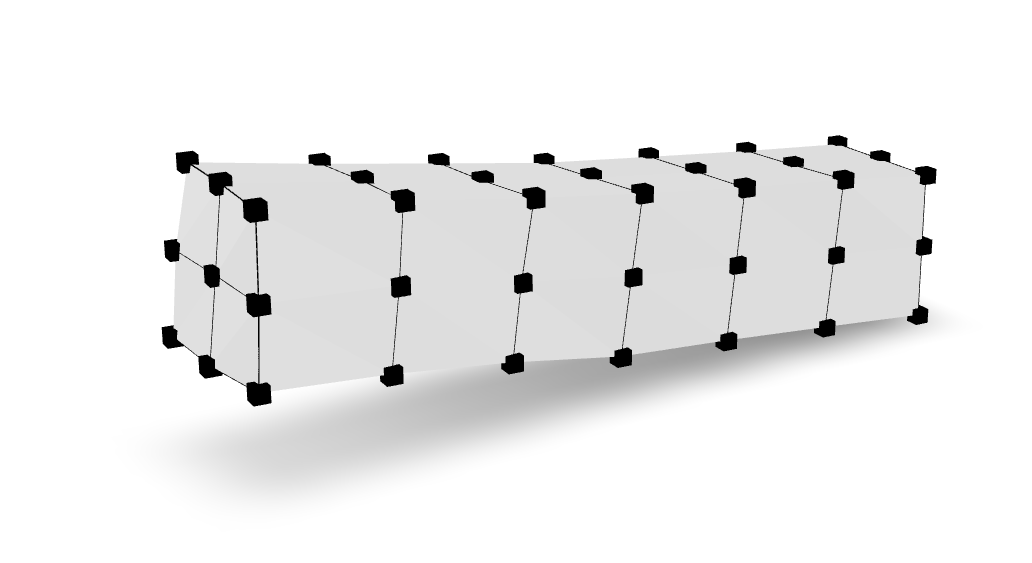
The deformed shape at the end of the analysis is rendered below:

The results consist of the file cantilever.out, which contains a line for every time step. Each line contains the time and the horizontal displacement at the upper right corner the beam. This is plotted in the figure below: