Flexible Rod Buckling Under Torque

3 min read • 445 words

Geometrically nonlinear analysis of a shaft buckling under torsion.

E50_Hockling.m

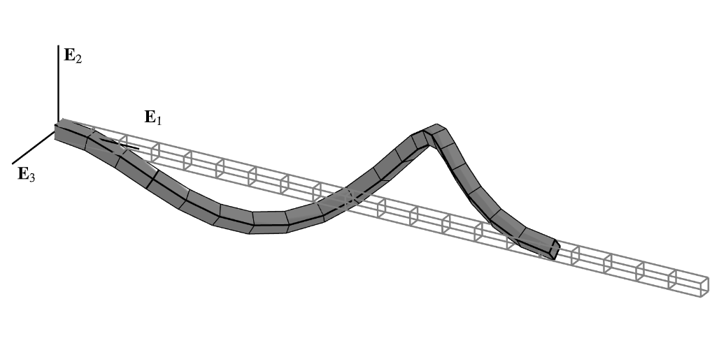
The hockling shaft (rendered above using the veux library) is a particularly complex problem that arises from practical considerations for the design of propeller shafts in large ships . This post follows from the work by . The problem is posed as a propped cantilever with a torque $T\,\mathbf{E}_1$ applied at its end $\xi = L$ . In OpenSees, this is defined as follows:

nn = ne + 1
T  = E*I/L
model.pattern("Plain", 1, "Linear", load={
    nn: [0, 0, 0,  T, 0, 0]
})

set T [expr $E*$I/$L]
pattern Plain 1 "Linear" {
    load $nn 0 0 0 $T 0 0
}

The rod is fixed at the origin and is free to translate along the $\mathbf{E}_1$ direction at its end.

This problem was investigated analytically by who found an approximate minimum buckling torque $T_{\mathrm{cr}}$ given by:

T_{\mathrm{cr}} = \lambda_{\text{cr}} \frac{2 EI}{L} \qquad\text{ where }\qquad \lambda_{\text{cr}} = \min \left\{\lambda \mid \tan \lambda - \lambda = 0\right\} \approx \pm 4.493409

reports the value $\lambda_{\text{cr}} \approx \pm 4.494$ , which is commonly used in the literature. Because the loaded end is constrained to rotate about a fixed axis, all rotation parameterizations coincide at this node so that, in all cases, the moment can be applied by simple scaling of a reference vector.

The following parameters are commonly adopted for the problem

\begin{array}{lcr} L &=& 240 \\ % ,& A &= 10 \\ E &=& 71240 \\ % ,& I &= 0.0833 \\ G &=& 27190 \\ % ,& J &= 2.16 \\ \end{array} \qquad\qquad \begin{array}{lcr} A &=& 10\hphantom{.0833} \\ I &=& 0.0833 \\ J &=& 2.16\hphantom{33} \\ \end{array}

To induce bifurcation, the undeformed centerline $\boldsymbol{x}_0(\xi)$ is slightly rotated off the axis of the roller reaction:

\boldsymbol{x}_0(\xi) = \xi \operatorname{Exp}\begin{pmatrix} 0 \\ 10^{-3} \\ 0 \end{pmatrix} \mathbf{E}_1 .

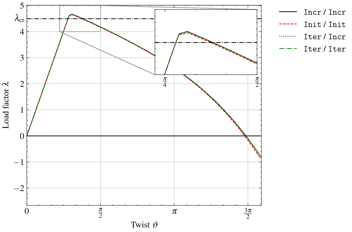
The simulation uses a discretization of 20 elements for the rod, and the torque is applied in 65 increments with iterative and incremental load factor control. The analysis uses the SFIN isometry with both None and Incr interpolation and parameterization variants. Figure 2 shows the relation between load factor $\lambda$ and end rotation $\vartheta = \|\operatorname{Log}\boldsymbol{\Lambda}(L)\|$ . This figure shows that the buckling load of the simulation is slightly higher than the value derived by , but is consistent with findings for geometrically exact elements in the literature .

$Relation between load factor λ\lambda and end rotation angle ϑ\vartheta for the hockling problem with the SFIN isometry and different interpolation/parameterization pairs.$

This investigation leveraged the FEDEASLab toolbox for nonlinear finite element analysis. Documentation is under development and expected to be published in Summer 2025. Source code for the geometric transformation framework is available on GitHub .

References

Finite Rotations

Force vs. Displacement formulations