Isoparametric Elements

8 min read • 1,526 words

A finite element analysis is performed of a plane beam with a hole using Lagrange quadrilaterals.

plane_block.py

This example introduces mesh-building tools for solid modeling. A finite element analysis is performed of a plane beam with a hole using various Lagrange quadrilaterals. Visualization is performed using the veux library.

Creating Blocks

Preliminaries

Before generating elements, we’ll first prepare our Model by defining an appropriate material and section. Each node of the analysis has two displacement degrees of freedom. Thus the model is defined with ndm = 2 and ndf = 2.

import opensees.openseespy as ops

model = ops.Model(ndm=2, ndf=2)

model -ndm 2 -ndf 2

As with the example of a tapered beam, the ElasticIsotropic material model is employed.

E = 4e3
nu = 0.25 # Poisson's ratio
model.material("ElasticIsotropic", 1, E, nu, 0)
model.section("PlaneStress", 1, 1, 1.0)

Quadrilateral Meshes

Next a mesh of quadrilateral elements is generated. The surface method is used as follows:

mesh = model.surface((nx, ny),
                  element=element,
                  args={"section": 1},
                  order=order,
                  points={
                    1: [  0.0,   0.0],
                    2: [   L,    0.0],
                    3: [   L,     d ],
                    4: [  0.0,    d ]
            })

where:

element is a string variable containing the name of the element type to generate.
order is an integer indicating the polynomial order of the generated elements; order=1 will create standard 4-node quadrilaterals, and order=2 will generate quadratic 9-node quadrilaterals.
nx and ny are integers indicating how many elements to create in the $x$ and $y$ directions.
args is a Python dictionary of arguments to be passed to each generated element. In this case the "section" keyword is used.

analysis script (collapsed)

# import the OpenSees Python module
import xara
import veux
import numpy as np
from xara.units.iks import kip, inch, foot, ksi
from xara.helpers import find_node, find_nodes
from veux.stress import node_average
from scipy.spatial.distance import euclidean as distance
import matplotlib.pyplot as plt
try:
    plt.style.use("veux-web")
except:
    pass

def create_beam(mesh,
                order=1,
                thickness=1,
                element: str = "LagrangeQuad"):

    nx, ny = mesh
    # Define geometry
    # ---------------
    E = 4000.0*ksi
    nu = 0.25
    L = 240.0*inch
    d = 24.0*inch
    thick = 1.0*inch
    load = -20.0*kip
    G = E / (2 * (1 + nu))
    A = thick*d
    k = 5/6
    w = load/L
    I = thick*d**3/12


    #
    # Create model
    #
    # create model in two dimensions with 2 DOFs per node
    model = xara.Model(ndm=2, ndf=2)

    # Define the material
    # -------------------
    #                                 tag     E      nu   rho
    model.material("ElasticIsotropic", 1, E, nu, 0)
    model.section("PlaneStress", 1, 1, thick)

    # now create the nodes and elements using the surface command
    # {"quad", "enhancedQuad", "tri31", "LagrangeQuad"}:


    mesh = model.surface((nx, ny),
                  element=element,
                  args={"section": 1},
                  order=order,
                  points={
                    1: [  0.0,   0.0],
                    2: [   L,    0.0],
                    3: [   L,     d ],
                    4: [  0.0,    d ]
            })

    # Single-point constraints
    #            x   (u1 u2)
    for node in find_nodes(model, x=0):
        model.fix(node, (1, 1))

    for node in find_nodes(model, x=L):
        model.fix(node, (1, 1))

    # Define gravity loads
    # create a Plain load pattern with a linear time series
    model.pattern("Plain", 1, "Linear")

    # Load all nodes with y-coordinate equal to `d`
    for nodes in mesh.walk_edge():
        # skip edges that arent on the top
        if abs(model.nodeCoord(nodes[0], 2) -d) < 1e-10:
            continue
        if abs(model.nodeCoord(nodes[-1], 1) -L) < 1e-10:
            continue
        if abs(model.nodeCoord(nodes[0], 1)) < 1e-10:
            continue

        # Edge length
        Le = distance(model.nodeCoord(nodes[0]), model.nodeCoord(nodes[-1]))

        if order == 1:
            model.load(nodes[0], (0,   w*Le/2), pattern=1)
            model.load(nodes[1], (0,   w*Le/2), pattern=1)
        elif order == 2:
            model.load(nodes[0], (0,   w*Le/6), pattern=1)
            model.load(nodes[1], (0, 2*w*Le/3), pattern=1)
            model.load(nodes[2], (0,   w*Le/6), pattern=1)

    #
    # Run Analysis
    #
    model.integrator("LoadControl", 1.0)
    model.analysis("Static")
    model.analyze(1)

    #
    # Beam theory solution
    #

    xn = [
         model.nodeCoord(node,1) for node in find_nodes(model, y=d/2)
    ]

    um = [
         model.nodeDisp(node, 2) for node in find_nodes(model, y=d/2)
    ]

    uy = lambda x: w*x**2/(24*E*I)*(L - x)**2 - w/(k*G*A)*L**2/24*(1 - 12*x/L + 12*(x/L)**2) + w*L**2/(24*G*A*k)
    ue = [uy(x) for x in xn]

    model.reactions()
    print(sum(model.nodeReaction(node, 2) for node in model.getNodeTags()))

    return model, xn, um, ue




if __name__ == "__main__":
    order = 2
    fig, ax = plt.subplots()
    for order in 1,2:
        # model, xn, um, ue = create_beam((40,8), element="quad", order=order)
        model, xn, um, ue = create_beam((12,4), element="quad", order=order)
        ax.plot(xn, um, ":", label=f"FEA ({order = })")

    ax.plot(xn, ue, label="Beam theory")

    ax.set_xlabel("Coordinate, $x$")
    ax.set_ylabel("Deflection, $u_y$")
    ax.legend()
    plt.savefig("img/beam_solution.png", dpi=300)
    plt.show()


    artist = veux.create_artist(model, canvas="gltf")

    stress = {node: stress["sxx"] for node, stress in node_average(model, "stressAtNodes").items()}

    artist.draw_nodes()
    artist.draw_outlines()
    artist.draw_surfaces(state=model.nodeDisp, scale=50, field=stress)
#   artist.draw_surfaces(field = stress)
    artist.draw_outlines(state=model.nodeDisp, scale=50)
    veux.serve(artist)


#       print(model.nodeDisp(l2))

Analysis

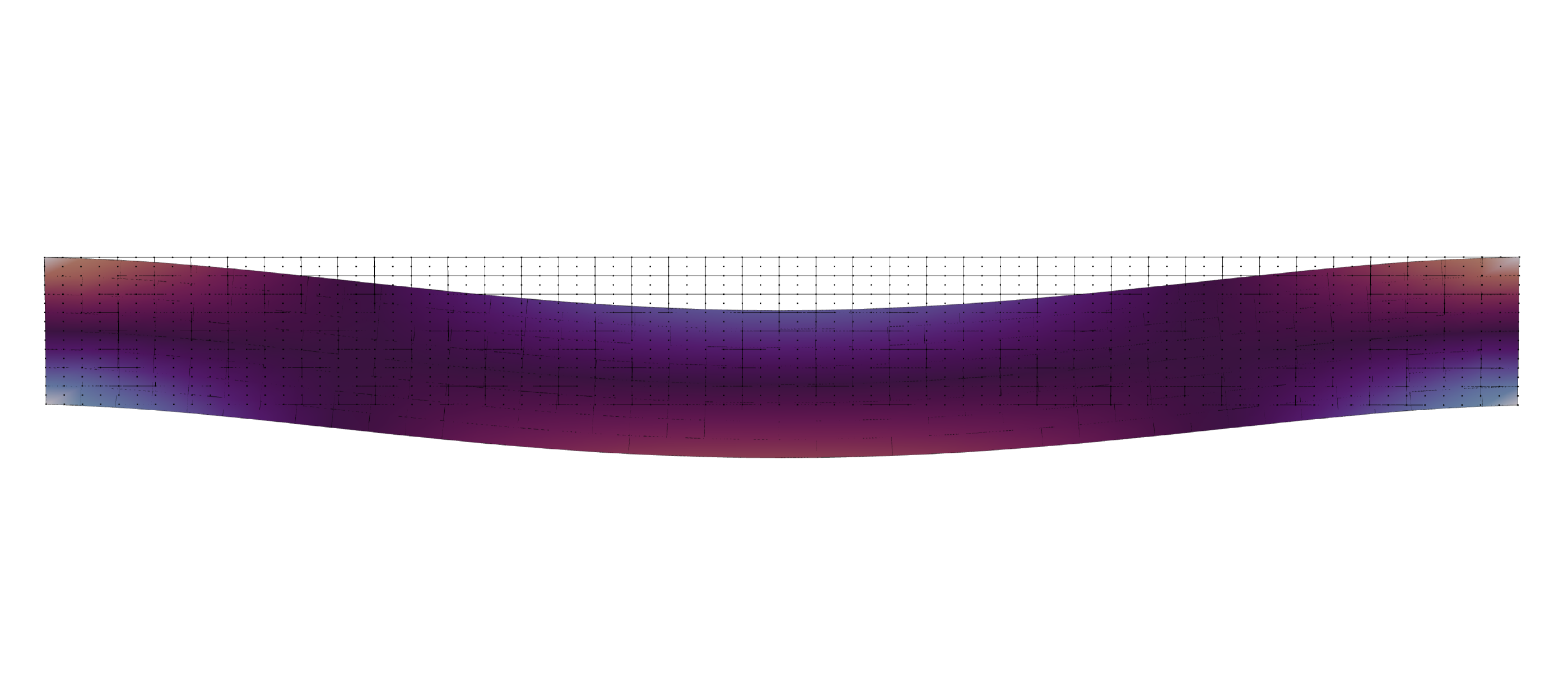
Validation

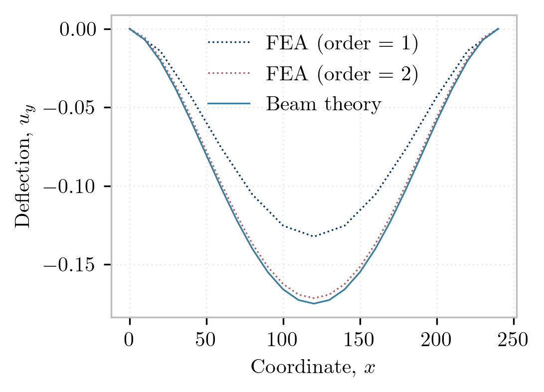
Consider the equilibrium differential equations for a 2D Timoshenko beam:

\begin{gathered} A G k_s\left( u_y'+\theta\right) - EI \theta'' =0 \\ -A G k_s\left(u_y''+ \theta'\right)=\bar{w} \end{gathered}

This is a coupled ODE for the displacement $u_y(x)$ and cross-section rotation $\theta(x)$ . The boundary conditions for this problem are

u_y(0)=0, \quad \theta(0)=0, \quad u_y(L)=0 \quad \theta(L)=0

and the solution is:

u_y(x)=\frac{q_0 L^4}{24 E I^{}} \frac{x^2}{L^2}\left(1-\frac{x}{L}\right)^2-\frac{1}{k_s G A}\frac{q_0 L^2}{24} \left(1-12 \frac{x}{L}+12 \frac{x^2}{L^2}\right) + \frac{1}{G A k_s L^2} \frac{q_0 L^4}{24}

This is plotted below along with the results of the finite element analysis with 4 and 9-node quadrilaterals:

Combining Blocks

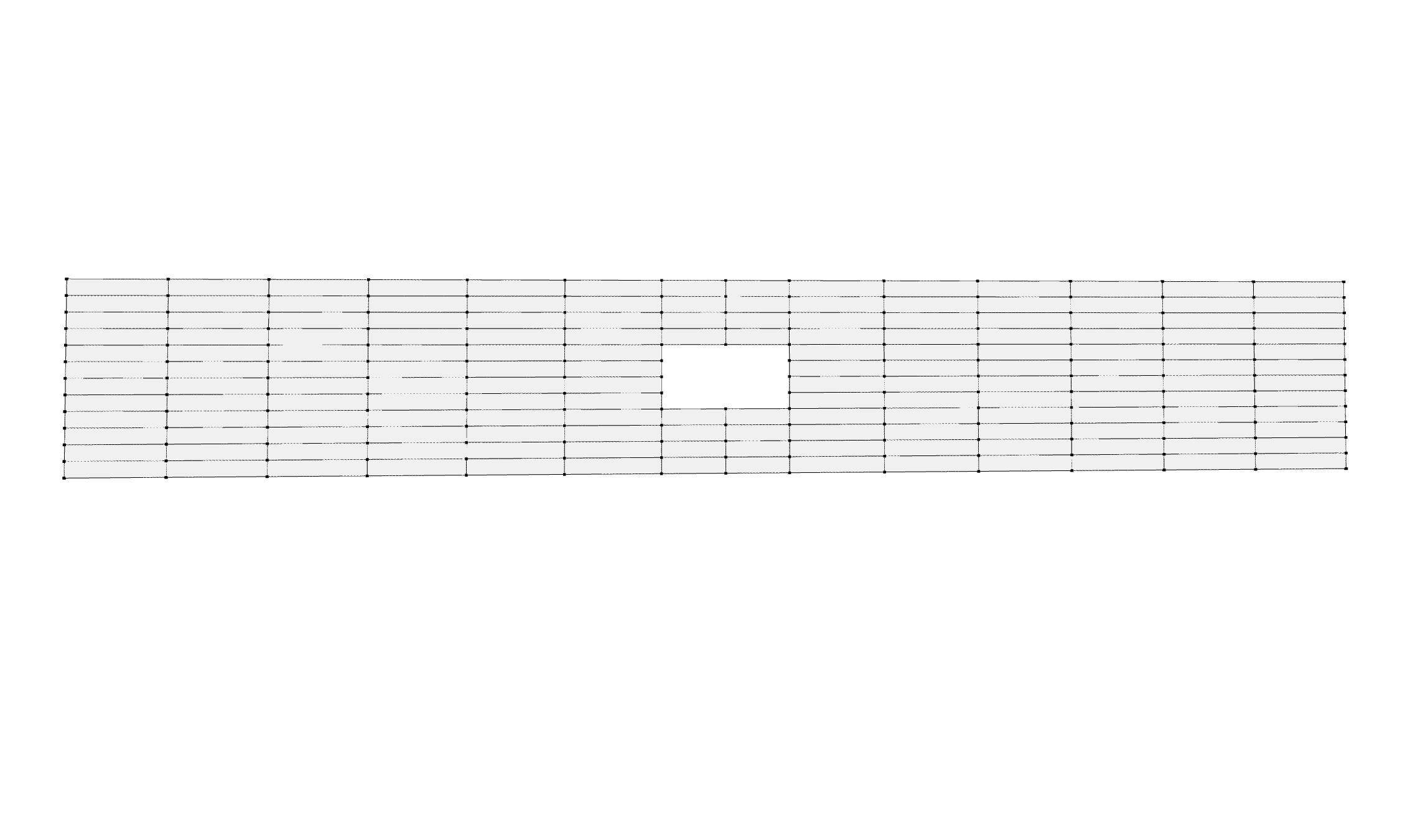
Now we will perform the same simulation, but with a hole cut into the beam. The shps package gives us more detailed control over the mesh generation process. The create_block function has the same basic functionality as the block2D method, but it doest actually add elements or nodes to a Model. Instead, it returns generated node coordinates (nodes) and cell connectivities (cells) as follows:

from shps import plane
from shps.block import create_block
points  = {
        1: (    0.0,   0.0),
        2: (L/2-w/2,   0.0),
        3: (L/2-w/2, d/2-h/2),
        4: (    0.0, d/2-h/2),
}
nodes, cells = create_block(ne, element, points=points)

It also exposes a join keyword argument which appends the generated nodes and cells to a given set of preexisting nodes and cells:

points  = {
        1: (L/2+w/2,   0.0),
        2: (   L   ,   0.0),
        3: (   L   , d/2-h/2),
        4: (L/2+w/2, d/2-h/2),
}
other = dict(nodes=nodes, cells=cells)
nodes, cells = create_block(ne, element, points=points, join=other)

This checks for duplications, and only adds nodes where none existed before. The following complete script is used to perform the complete simulation.

analysis script (collapsed)

import xara
import veux
from xara.helpers import find_node, find_nodes
from veux.stress import node_average
from shps import plane
from shps.block import create_block


def hole(order):
    d = 24   # Beam depth
    L = 240  # Beam length
    h =  8   # Hole height
    w = L/6  # Hole width
    ne = 6,4

    # Define the element type; first-order Lagrange quadrilateral
    element = plane.Lagrange(order)
    points  = {
            1: (    0.0,   0.0),
            2: (L/2-w/2,   0.0),
            3: (L/2-w/2, d/2-h/2),
            4: (    0.0, d/2-h/2),
    }
    nodes, cells = create_block(ne, element, points=points)
#
    points  = {
            1: (L/2+w/2,   0.0),
            2: (   L   ,   0.0),
            3: (   L   , d/2-h/2),
            4: (L/2+w/2, d/2-h/2),
    }
    other = dict(nodes=nodes, cells=cells)
    nodes, cells = create_block(ne, element, points=points, join=other)
#
    points  = {
            1: (L/2+w/2, d/2-h/2),
            2: (   L   , d/2-h/2),
            3: (   L   , d/2+h/2),
            4: (L/2+w/2, d/2+h/2),
    }
    other = dict(nodes=nodes, cells=cells)
    nodes, cells = create_block(ne, element, points=points, join=other)

#
    points  = {
            1: (L/2+w/2, d/2+h/2),
            2: (   L   , d/2+h/2),
            3: (   L   , d    ),
            4: (L/2+w/2, d    ),
    }
    other = dict(nodes=nodes, cells=cells)
    nodes, cells = create_block(ne, element, points=points, join=other)
#
    points  = {
            1: (  0.0  , d/2+h/2),
            2: (L/2-w/2, d/2+h/2),
            3: (L/2-w/2, d      ),
            4: (  0.0  , d      ),
    }
    other = dict(nodes=nodes, cells=cells)
    nodes, cells = create_block(ne, element, points=points, join=other)
#
    points  = {
            1: (  0.0  , d/2-h/2),
            2: (L/2-w/2, d/2-h/2),
            3: (L/2-w/2, d/2+h/2),
            4: (  0.0  , d/2+h/2),
    }
    other = dict(nodes=nodes, cells=cells)
    nodes, cells = create_block(ne, element, points=points, join=other)
#
    ne = 2,4
    points  = {
            1: (L/2-w/2, d/2+h/2),
            2: (L/2+w/2, d/2+h/2),
            3: (L/2+w/2, d      ),
            4: (L/2-w/2, d      ),
    }
    other = dict(nodes=nodes, cells=cells)
    nodes, cells = create_block(ne, element, points=points, join=other)
# 
    points  = {
            1: (L/2-w/2,   0.0),
            2: (L/2+w/2,   0.0),
            3: (L/2+w/2, d/2-h/2),
            4: (L/2-w/2, d/2-h/2),
    }
    other = dict(nodes=nodes, cells=cells)
    nodes, cells = create_block(ne, element, points=points, join=other)
#
    return nodes, cells

def create_model(mesh,
                thickness=1,
                element: str = "LagrangeQuad"):
    # Define geometry
    # ---------------

    L = 240.0
    d = 24.0
    thick = 1.0
    load = 20.0 # kips


    # create model in two dimensions with 2 DOFs per node
    model = xara.Model(ndm=2, ndf=2)

    # Define the material
    # -------------------
    #                                 tag  E      nu   rho
    model.material("ElasticIsotropic", 1, 4000.0, 0.25, 0, "-plane-strain")

    # now create the nodes and elements
    args = (thick, "PlaneStrain", 1)

    for tag, node in mesh[0].items():
        model.node(tag, *node)

    for tag, cell in mesh[1].items():
        model.element(element, tag, tuple(cell), *args)

    # Fix all nodes with coordinate x=0.0
    for node in find_nodes(model, x=0):
        #         tag   (u1 u2)
        model.fix(node, (1, 1))

    # Fix all nodes with coordinate x=L
    for node in find_nodes(model, x=L):
        model.fix(node, (1, 1))

    # Define gravity loads
    # create a Plain load pattern with a linear time series
    model.pattern("Plain", 1, "Linear")

    # Load all nodes with y-coordinate equal to `d`
    top = list(find_nodes(model, y=d))
    for node in top:
        model.load(node, (0.0, -load/len(top)), pattern=1)

    return model


def static_analysis(model):

    # Define the load control with variable load steps
    model.integrator("LoadControl", 1.0)

    # Declare the analysis type
    model.analysis("Static")

    # Perform static analysis in 10 increments
    model.analyze(10)


if __name__ == "__main__":
    import time

    mesh = hole(1)
    model = create_model(mesh, element="quad")
    start = time.time()
    static_analysis(model)
    print(f"Finished {time.time() - start} sec")
    print(model.nodeDisp(find_node(model, x=240, y=0)))


    artist = veux.create_artist(model)

    stress = {node: stress["sxx"] for node, stress in node_average(model, "stressAtNodes").items()}

    artist.draw_surfaces(state=model.nodeDisp, field = stress, scale=10)
    artist.draw_outlines()
    veux.serve(artist)

Inelastic Plane Frame

Frame with Diaphragms

On this page: