Plane Tapered Cantilever

3 min read • 535 words

A finite element analysis is performed of a plane tapered cantilever using constant-strain triangles.

plane_taper.py

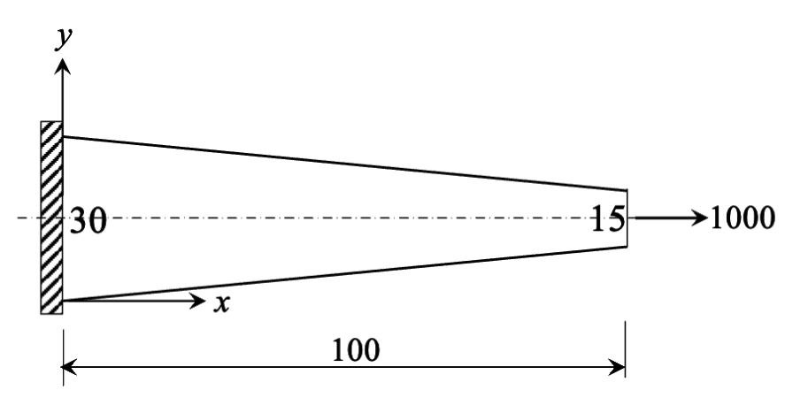
A finite element analysis is performed of a plane tapered cantilever using constant-strain triangles. The ElasticIsotropic material model is employed. Visualization is performed in the script render.py using the veux library.

Once again the surface method is used to generate the finite element mesh. However, in the present study we omit the element argument so that only nodes are generated:

mesh = model.surface((nx, ny),
              points={
                1: [  0.0,   0.0],
                2: [   L,    L*r],
                3: [   L,  b-L*r],
                4: [  0.0, b    ]
              })

The resulting mesh variable is then used to manually construct the triangular elements:

elem = 1
for cell in mesh.cells:
    nodes = mesh.cells[cell]
    model.element("tri31",   elem, [nodes[0], nodes[1], nodes[2]], section=1)
    model.element("tri31", elem+1, [nodes[0], nodes[2], nodes[3]], section=1)
    elem += 2

Note that care must be taken to apply the distributed load at the tip in a consistent manner. For elements with linear interpolation at the boundary one has:

from xara.helpers import find_node, find_nodes

tip = list(find_nodes(model, x=L))
for node in tip:
    px = load/len(tip)

    # Divide load at edges by two
    if abs(model.nodeCoord(node, 2)) in {7.5, 22.5}:
        px /= 2
    model.load(node, (px, 0.0), pattern=1)

where we’ve used the find_nodes helper function from the xara.helpers module.

The stress field looks like:

analysis script (collapsed)

#
# Tapered cantilever beam
#
# Description
# -----------
#  Tapered cantilever beam modeled with two dimensional solid elements
# 
# Objectives
# ----------
#  Test different plane elements
#
import veux
import xara
from xara.helpers import find_node, find_nodes
from veux.stress import node_average


def create_model(mesh,
                 thickness=1,
                 element: str = "LagrangeQuad"):

    nx, ny = mesh

    # create model in two dimensions with 2 DOFs per node
    model = xara.Model(ndm=2, ndf=2)

    # Define the material
    # -------------------
    #                                 tag    E      nu   rho
    model.material("ElasticIsotropic", 1, 10_000.0, 0.25, 0)
    model.section("PlaneStress", 1, 1, thickness)

    # Define geometry
    # ---------------

    load = 1000.0
    b = 30
    L = 100.0
    r = (b/4)/L

    # Create the nodes and elements using the surface command
    args = ("-section", 1)

    mesh = model.surface((nx, ny),
                  points={
                    1: [  0.0,   0.0],
                    2: [   L,    L*r],
                    3: [   L,  b-L*r],
                    4: [  0.0, b    ]
                  })
    elem = 1
    for cell in mesh.cells:
        nodes = mesh.cells[cell]
        model.element("tri31",   elem, [nodes[0], nodes[1], nodes[2]], section=1)
        model.element("tri31", elem+1, [nodes[0], nodes[2], nodes[3]], section=1)
        elem += 2

    # Single-point constraints
    #            x   (u1 u2)
    for node in find_nodes(model, x=0.0):
        print("Fixing node ", node)
        model.fix(node, (1, 1))

    # Define gravity loads
    # create a Plain load pattern with a linear time series
    model.pattern("Plain", 1, "Linear")

    # Find the node at the tip center

    tip = list(find_nodes(model, x=L))
    for node in tip:
        px = load/len(tip)

        # Divide load at edges by two
        if abs(model.nodeCoord(node, 2)) in {7.5, 22.5}:
            px /= 2
        model.load(node, (px, 0.0), pattern=1)

    return model



def static_analysis(model):

    # Define the load control with variable load steps
    model.integrator("LoadControl", 1.0)

    # Declare the analysis type
    model.analysis("Static")

    # Perform static analysis
    model.analyze(1)



if __name__ == "__main__":
    import time
    for element in "quad", : # "LagrangeQuad", "quad":
#       model = create_model((20,6), element=element)
        model = create_model((40,10), element=element)
#       model = create_model((80,10), element=element)
        start = time.time()
        static_analysis(model)
        print(f"Finished {element}, {time.time() - start} sec")
        print(model.nodeDisp(find_node(model, x=100, y=15)))



    artist = veux.create_artist(model) #, model.nodeDisp, scale=10)

    stress = {node: stress["sxx"] for node, stress in node_average(model, "stressAtNodes").items()}

    artist.draw_surfaces(field = stress)
    artist.draw_outlines()
    veux.serve(artist)

Linearized Buckling

Pure flexure